By Fabio Marini in databases — May 1, 2022

PostgreSQL with Apache AGE - Playing more seriously with Graph Databases

Making something useful with a graph database, beyond the basic stuff. Creating multiple nodes and relationships and navigating the graph

Photo by Conny Schneider / Unsplash

In my initial post about PostgreSQL and Apache AGE I spent some time discussing the pros and cons of the technology and why it can be a great addition to the developer's toolbox. In this post, we will explore more features of the Apache AGE extension and the power of the OpenCypher query language.

Status of the technology

Before we start exploring the power of AGE let's talk about the status of the project. If you have a look at the GitHub project page, the first thing you notice from the URL is that we are approaching version 1.0.0 but the entire project is still in the Apache Incubator phase, so it's not yet a mainstream project.

Don't get me wrong, I'm not meaning you should be scared or keep away from it, you just need to be careful when using AGE for your projects, and remember that a young project is likely subject to big changes, often with little to no backward compatibility. This is happening in each release at the moment since the APIs are still getting stabilized and optimized, and when you upgrade for example from release 0.7 to 1.0.0 there is no real upgrade path.

To keep experimenting during this phase of heavy development, I prefer using the Docker image and moving my data in and out from one release to the other. Sure this is not a safe nor nice way of working, since the risk of losing some data is still present, but I'm planning to use AGE in a real project that is in its infancy right now, so the time could be just right to get to a production release of both at the same time.

Even with these premises, the technology is already pretty solid and you can use it safely for some serious graph development.

Running AGE inside Docker (on Apple Silicon)

Side note: I recently moved to a new MacBook Pro with the Apple M1 Pro processor, and I have to admit that I'm loving it very much. I was worried about having a bunch of problems with the migration but as of now, aside from Virtual Machines for x86 that are incompatible with Apple Silicon by design, I've yet to find any issue with the new hardware. To be honest, I'm impressed by the performance difference over my previous 2019 MacBook Pro with Intel i9, I'm really happy to see serious competition to Intel's monopoly in the CPU market.

That said, the "official" Docker image for Apache AGE is still built for the Intel architecture, and even if it works flawlessly with my M1 Pro, I still prefer to have a native image to play with, so let's see how to build it from sources.

To create a build of AGE from sources, you just need to clone the repository locally and launch the Docker build command. At the moment I found that a dependency has changed inside the base Debian Stretch image used by the base Postgres:11 image, so you need a small change to the Dockerfile.

Open it in your editor and change the FROM line from:

FROM postgres:11
...

The original Dockerfile

FROM postgres:11-bullseye
...

The patched Dockerfile

This changes the base image from Debian Stretch to Debian Bullseye where the postgresql-server-dev-11 package is available.

After changing the Dockerfile open the terminal and run the following command to build the image:

docker build -t sorrell/apache-age .

The Docker build command

I kept the sorrell/apache-age tag that is the same as the official image so that I can swap it with a new official image whenever it will be available.

At the end of the build process the new AGE Docker image is ready to play with, and in my case, also built for my hardware architecture.

When running dockerized database images, I prefer to keep the data outside the container so that I can upgrade the image version while preserving the content. For that reason, I use a local ./db-data folder mounted as a volume for the container. The service is then run using Docker Compose with the following definition:

version: "3.3"
services:
  db:
    image: sorrell/apache-age
    environment:
      - POSTGRES_PASSWORD=P@s5W0rd$
    ports:
      - 5432:5432
    volumes:
      - ./db-data:/var/lib/postgresql/data

The docker-compose.yml for Apache AGE

To start the service, from the folder where your docker-compose.yml file is stored, you can run the following command:

docker-compose up

Connecting to the database

After the startup process is completed you are ready to start playing with AGE inside your preferred SQL tool. I usually use DBeaver for this or the Database Console inside IntelliJ Idea while I'm writing code.

The connection is the standard PostgreSQL one, but to get AGE to work we need some additional configuration. It is possible to set the search path in the connector parameters, or they can be specified directly after the connection is established.

CREATE EXTENSION IF NOT EXISTS age;
LOAD 'age';
SET search_path = ag_catalog, "$user", public;

Here we defined the age extension and loaded it, and we set the search path including ag_catalog to have the internal functions of AGE available without the need of prefixing them with the schema name.

Playing with the graph

Now that the database is ready let's play with it by creating a graph and putting some data inside it. In AGE each graph has its own schema inside Postgres, and the first thing to do before we can do anything is to create the graph.

SELECT create_graph('playground');

Now the graph is ready to be populated, and we have two possible ways of working:

define the structure of the graph by populating it with nodes and relations
create the structures for each node and relation beforehand

The first path is more dynamic so that you can define your graph while using it. This is a fast way, but you have to keep in mind that you cannot query things that don't yet exist. Like a relational database in fact, each node and relation is translated into one or more tables in the Postgres schema, and if you query a node with a specific label before creating it, the cypher query will return an error. That's why if you have your schema already defined it could be better to create all the structures before starting to populate them.

To create vertexes (nodes) and edges (relations) you can use the following functions:

-- Vertex definition
select create_vlabel(GRAPH_NAME,LABEL);

-- Edge definition
select create_elabel(GRAPH_NAME,LABEL);

An example schema

Let's imagine that we'd like to use AGE to model a basic product catalog.

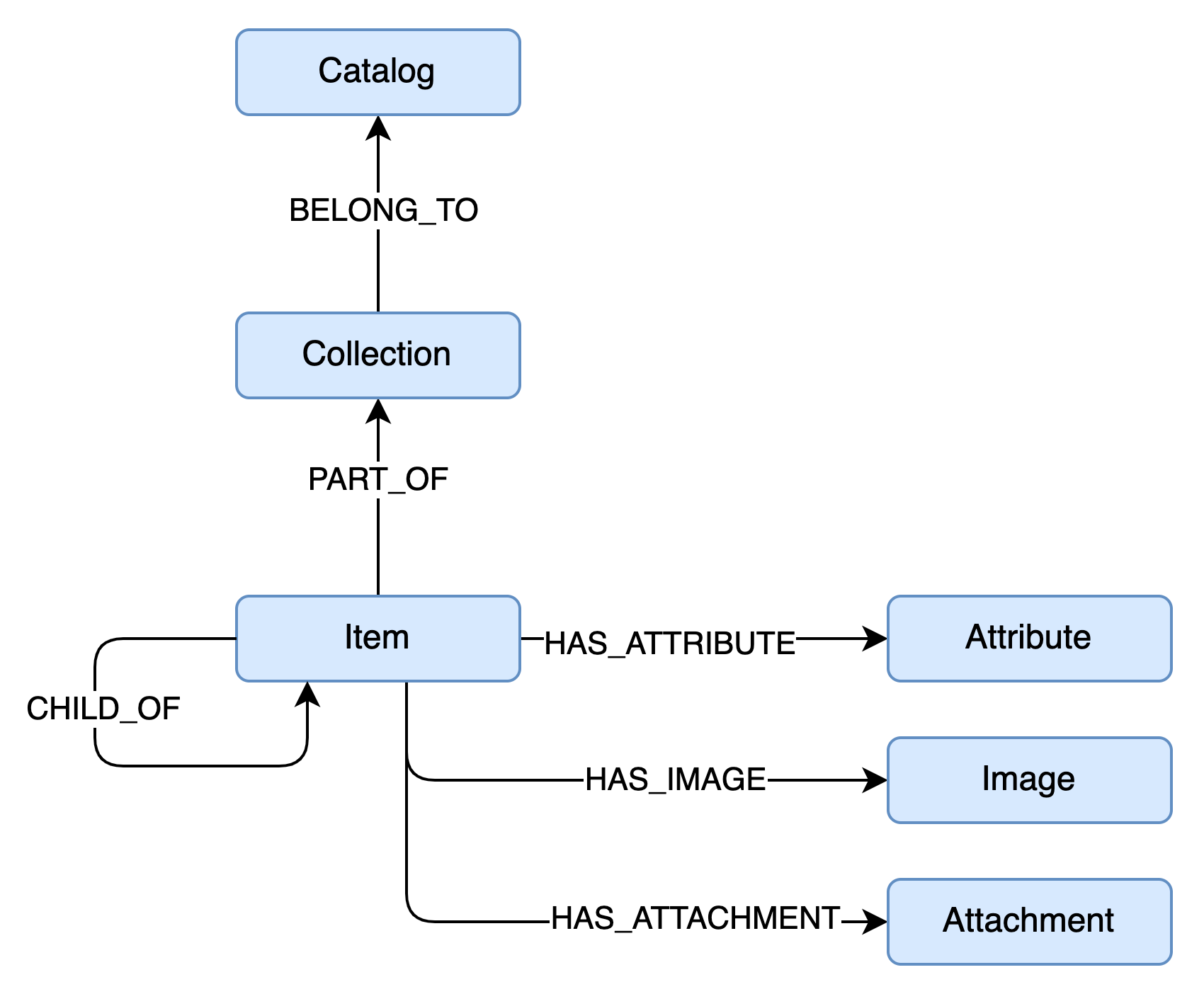
We can create one or more catalogs, for example, an apparel one, and inside it, we want to manage collections, for example, the spring-summer and the fall-winter ones. Every collection is then made of items that can have sub items, and each item has its own attributes, images and attachments.

Each entity in this schema (the blue rectangles) can be translated into a Node or Vertex, and each relationship between nodes is then translated to a Relation or Edge inside the graph. As a convention, we'll use PascalCase for node labels (i.e. Catalog) and all upper snake case for relations (i.e. HAS_ATTRIBUTE).

Now that we know all our nodes and relations, we can start defining them inside the graph.

-- Nodes
select create_vlabel('playground','Catalog');
select create_vlabel('playground','Collection');
select create_vlabel('playground','Item');
select create_vlabel('playground','Attribute');
select create_vlabel('playground','Image');
select create_vlabel('playground','Attachment');

-- Relations
select create_elabel('playground','BELONG_TO');
select create_elabel('playground','PART_OF');
select create_elabel('playground','CHILD_OF');
select create_elabel('playground','HAS_ATTRIBUTE');
select create_elabel('playground','HAS_IMAGE');
select create_elabel('playground','HAS_ATTACHMENT');

Graph structure definition

As you can see, for relations we don't need to specify the connections, but just the label. The connection is then handled by the actual data.

A look under the hood

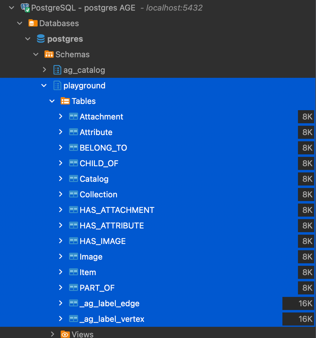
If we now have a look inside PostgreSQL, we will see that for each node and relation we created, AGE has defined a table to store the data. In addition to these tables there are also two generic _ag_label_edge and _ag_label_vertex.

In addition to these tables inside the playground schema (the name of the graph we created), there is an internal ag_catalog schema used by AGE to store the details of the graph.

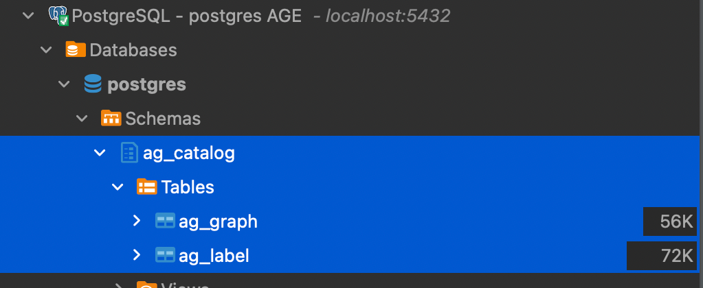
The ag_graph table stores the information about the existing graphs, in our case there is one record referring to our playground graph.

The ag_label table contains one record for each table in our graph schema and the information about its function (edge or vertex) and the connection to the graph and the actual table.

Every vertex table is then defined by two columns, id and properties. The id is the internal ID of the record, while the properties are the internal "hashmap" in which you can store additional information for the node.

Every edge table is defined by four columns, id, start_id, end_id and properties. The id and properties columns have the same function of the same inside the node tables, while the start_id and end_id are the links to the ids of the nodes connected by the edge.

Filling the graph with some data

Now that we defined the schema and had a look under the hood at how things work, let's see how to fill the graph with some data about our catalog.

Creating the catalog

To create a node in our graph we can use the CREATE instruction of the OpenCypher language that AGE use (not every feature of Cypher is implemented at the moment). Since AGE works as an extension to PostgreSQL, the main language is SQL, and the Cypher part of the query is wrapped inside the cypher function.

select * from cypher('playground', $$
    CREATE (c:Catalog { code: "C001" })
    SET c.name = "Apparel Catalog"
    RETURN c
$$) as (catalog agtype);

This instruction creates a new node with the Catalog label and a property named code and value C001, then modifies the node adding a name property with value Apparel Catalog and returns the node just created.

The output of the command is the following:

{"id": 844424930131969, "label": "Catalog", "properties": {"code": "C001", "name": "Apparel Catalog"}}::vertex

As you can see, AGE created the node with the label Catalog, assigned it an id and set our additional properties inside the properties field, just as expected.

If you remember, when we created the graph schema and label definitions, we never defined some sort of primary key, and this is because in AGE there are no custom indexes (at least at the moment). This means that we have no "referential integrity" we are used to in traditional relational databases. In fact, if you try to run the same create query again you will get two identical nodes.

This opens up a new problem, we need to be careful when creating objects inside the graph otherwise we will end up with a lot of duplicates not connected to the right node and this will render the entire graph useless.

To "fix" this problem in Cypher there is a second way of creating objects, the MERGE instruction. Merge is like an UPSERT instruction meaning that it looks for a pattern and if it doesn't exist, it creates the required nodes.

Take the following example:

select * from cypher('playground', $$
    MERGE (c:Catalog { code: "C001" })
    RETURN c
$$) as (catalog agtype);

This checks if a node with a label Catalog and code equals to C001 exists in the graph, and if it doesn't, it creates it.

In this case we can't use the SET instruction that is similar to an UPDATE, but we need to split it into two separate commands:

one to create the node with the code property set to our "primary key"
one to set the additional properties

select * from cypher('playground', $$
    MERGE (c:Catalog { code: "C001" })
    RETURN c
$$) as (catalog agtype);

select * from cypher('playground', $$
    MATCH (c:Catalog { code: "C001" })
    SET c.name = "Apparel Catalog"
    RETURN c
$$) as (catalog agtype);

This way we can work around the missing index and ensure that the node is created only once.

You could be tempted to put all of your custom properties inside the MERGE instruction, but this is wrong, because as said, AGE works by pattern matching, so if you use more than just the key properties, you could end up duplicating the nodes just because the already existing one has a property with a different value.

So use the MERGE instruction with just the key property and then update the nodes or edges with the MATCH .. SET instruction.

Adding a collection to the catalog

Now that we have our catalog inside the graph, let's create a collection and connect it to the parent catalog with the BELONG_TO relationship.

select * from cypher('playground', $$
    MATCH (c:Catalog { code: "C001"} )
    MERGE (co:Collection { code: "SS22" })
    MERGE (co)-[:BELONGS_TO]->(c)
    RETURN co
$$) as (collection agtype);

In the example, we looked for the Catalog with code C001 keeping the reference in a variable c, then we created the Collection with code SS22 and the relationship between the two using the MERGE (co)-[:BELONG_TO]->(c) instruction.

One of the nice aspects of the Cypher language is that it is pretty graphical, in fact, it is quite clear that there is an oriented relationship between the Collection and the Catalog just by looking at the instruction.

Adding a couple of items to the collection

Let's now add a couple of items to the SS22 collection.

select * from cypher('playground', $$
    MATCH (co:Collection { code: "SS22" })
    MERGE (i1:Item { code: 'ISS001'}) 
    MERGE (i1)-[:PART_OF]->(co)
    MERGE (i2:Item { code: 'ISS002'}) 
    MERGE (i2)-[:PART_OF]->(co)
    MERGE (i3:Item { code: 'ISS003'}) 
    MERGE (i3)-[:PART_OF]->(co)
    RETURN [i1, i2, i3]
$$) as (items agtype);

Here we can see another useful feature of Cypher, the possibility to have multiple instructions inside a single query. In the example, we are creating three different Item nodes and connecting each with the SS22 collection.

Now things can get more interesting. Let's say we want to retrieve all the items inside the C001 catalog, we can do this with the explicit pattern matching as follows:

select * from cypher('playground', $$
    MATCH (c:Catalog { code: "C001" })<-[:BELONGS_TO]-(co:Collection)<-[:PART_OF]-(i:Item)
    RETURN i
$$) as (item agtype);

but we can also use a more compact and powerful representation, variable length paths. Take the following example:

select * from cypher('playground', $$
    MATCH (c:Catalog { code: "C001" })-[*]-(i:Item)
    RETURN i
$$) as (item agtype);

This tells the graph to return all the Items that have someway relation of arbitrary length with the catalog C001. This is where the power of graph databases can surpass the traditional relational model. This kind of query in a traditional model is really complex if not even impossible to accomplish, and forces you to design the data model for this kind of query with a lot of trade-offs.

Of course, this kind of unconstrained path matching should be used very carefully because on a huge graph, the complexity can explode, and with it also the time and resources needed to get the results.

Updating items

Now that we created a couple of items inside the collection, let's update them with some attributes. In the example the attributes are separate nodes connected to Item, so how do we handle them? In a way similar to what we did for collection and items: using a combination of MATCH and MERGE.

select * from cypher('playground', $$
    MATCH (i:Item)
    WHERE i.code = "ISS001"
    SET i.name = "T-Shirt"
    MERGE (i)-[:HAS_ATTRIBUTE { value: "S"}]->(:Attribute { name: "size" })
    RETURN i
$$) as (item agtype);

In the example we do many things in a single query:

we look for the Item with code = ISS001, this time using the WHERE clause that is very similar to the SQL counterpart
we update the Item with a property name with value T-Shirt
we then create an Attribute named size and connect it to the Item via an HAS_ATTRIBUTE relationship that also has a property named value with value S

This multiple-instruction capability is another useful feature of the Cypher language. Let's now add the color attribute to the item, this time with a single MERGE instruction.

select * from cypher('playground', $$
    MERGE (i:Item { code: "ISS001"})-[:HAS_ATTRIBUTE { value: "Blue"}]->(:Attribute { name: "color" })
    RETURN i
$$) as (item agtype);

If you noticed, in a graph also the edges can have properties, and this is because relations are first-class citizens inside a graph, and they carry the same if not more information than the nodes they connect.

Retrieving values from the graph

Now that we have a bunch of vertexes and edges in place, let's see how to get the information out of the graph. We previously saw how to get the Items of a Catalog but we retrieved the entire Vertex structure. In this case, we want to look for all the attributes of the ISS001 Item but we are interested only in the name and value pairs.

select * from cypher('playground', $$
    MATCH (:Item { code: 'ISS001'})-[v:HAS_ATTRIBUTE]->(a:Attribute)
    RETURN a.name, v.value
$$) as (name agtype, value agtype);

The result is the following:

name	value
"size"	"S"
"color"	"Blue"

You will notice that the values are surrounded by double quotes, and this is because AGE works with its own data type agtype that is a superset of JSON so the values you get in the results are JSON structures, in this case, JSON strings. You need to keep this in mind because you'll need to decode the value to remove the double quotes if you need the plain string content.

Another interesting feature of AGE and the Cypher language is that you can create custom return values, so for example, instead of returning the name and value pairs, we can ask the graph to return a list of JSON objects with the name and value properties with a query like this.

select * from cypher('playground', $$
    MATCH (:Item { code: 'ISS001'})-[v:HAS_ATTRIBUTE]->(a:Attribute)
    RETURN {
        name: a.name,
        value: v.value
    }
$$) as (attr agtype);

The result of the previous query will be the following:

attr
{"name": "size", "value": "S"}
{"name": "color", "value": "Blue"}

Playing with AGE in Java with MyBatis

As discussed in previous posts, for my work projects I usually use Java with Spring Boot and MyBatis. Since AGE has custom data types, MyBatis requires some additional customization to manage the results of the Mappers.

To help with this I created a small utility library that fills the gap and helps in using MyBatis with Apache AGE in a quite simple way.

Feel free to try it and if you have some questions you can open an issue directly on GitHub or contact me on Twitter @FabioMariniNet

Next steps

We still just scratched the surface of what a graph database can do, but we now have more knowledge of how things work inside AGE and how data are handled inside the Postgres schemas.

In future articles, we will go deeper into the model and try to see some more additional and powerful features of graph databases and AGE in particular.

Stay tuned for the next episodes.